Binary metric A/B test design example using Ambrosia
This example is about how Ambrosia can be used to calculate the parameters of an experiment with binary metrics. For a binary metric, there are some differences in the calculations regarding continuous metrics.
Let’s consider an example of calculating the parameters of a hypothetical experiment based on synthetic data on user retention rate.
[2]:
import numpy as np
import pandas as pd

import matplotlib.pyplot as plt
import seaborn as sns

from ambrosia.designer import Designer, design_binary
Load data
[3]:
data = pd.read_csv('../tests/test_data/ltv_retention.csv')
[4]:
data.head()
[4]:
| LTV | retention | |
|---|---|---|
| 0 | 38.004891 | 0.0 |
| 1 | 70.588069 | 1.0 |
| 2 | 13.585602 | 1.0 |
| 3 | 19.813550 | 0.0 |
| 4 | 207.213003 | 0.0 |
Experiment design based on available historical data
In many situations, we have historical retention/conversion rate data available, and this data can be used in the same way as continuous data.
In order to calculate some A/B test parameters of interest, such as experimental power, group size, or minimum detectable effect, we need to pass them in the same way to the Designer class.
[5]:
designer = Designer(dataframe=data, metrics='retention')
For binary data, we can use either the "theory" method or the "binary" method.
"theory" method performs a numerical calculation of the parameters using various approximations.stabilizing_method parameter and defaults to "asin" which is more accurate and robust. You can find more information about the approximations on the Net."binary" approach does parameter estimation based on the multiple construction of chosen confidence interval. Some of these intervals are quite exotic and should be studied for conscious application. As a default a standard Wald interval is used.Now let’s create a grid of known parameters and calculate interested ones. We will use two above methods consequntly.
[6]:
# Create grid of MDEs and group sizes
# I and II type errros will have default values
effects = [1.02, 1.05, 1.1]
group_sizes = [500, 1000, 2000]
First design group sizes
[7]:
designer.run(to_design='size', method='theory', effects=effects)
[7]:
| Errors ($\alpha$, $\beta$) | (0.05; 0.2) |
|---|---|
| Effect | |
| 2.0% | 58885 |
| 5.0% | 9464 |
| 10.0% | 2382 |
Then design MDE values
[8]:
designer.run(to_design='effect', method='theory', sizes=group_sizes)
[8]:
| Errors ($\alpha$, $\beta$) | (0.05; 0.2) |
|---|---|
| Group sizes | |
| 500 | 21.9% |
| 1000 | 15.5% |
| 2000 | 10.9% |
Finally design power
[9]:
designer.run(to_design='power',
             method='theory',
             effects=effects,
             sizes=group_sizes)
[9]:
| Group sizes | 500 | 1000 | 2000 | |
|---|---|---|---|---|
| $\alpha$ | Effect | |||
| 0.05 | 2.0% | 5.8% | 6.5% | 8.1% |
| 5.0% | 9.9% | 14.9% | 25.1% | |
| 10.0% | 25.0% | 44.3% | 72.8% |
"binary" approach and compare to "theory" method result.amount parameter to check how the accuracy of estimated group size value is increased[10]:
interval_amounts = [2000, 5000, 20000]
group_size_estimation_dict = {}
[11]:
for amount in interval_amounts:
    group_size_estimation_dict[amount] = []
    for step in range(200):
        estimated_size = designer.run(to_design='size',
                                      method='binary',
                                      interval_type='wald',
                                      amount=amount,
                                      effects=1.1).values[0][0]
        group_size_estimation_dict[amount].append(estimated_size)
Draw the results
[12]:
plt.figure(figsize=(8, 6))
plt.title('Group size estimation for 10% MDE')
for key in group_size_estimation_dict:
    label = f'amount number={key}'
    sns.histplot(group_size_estimation_dict[key], label=label)
plt.plot(2382, 0.5, 'ro', label='Theoretical estimation')
plt.legend();
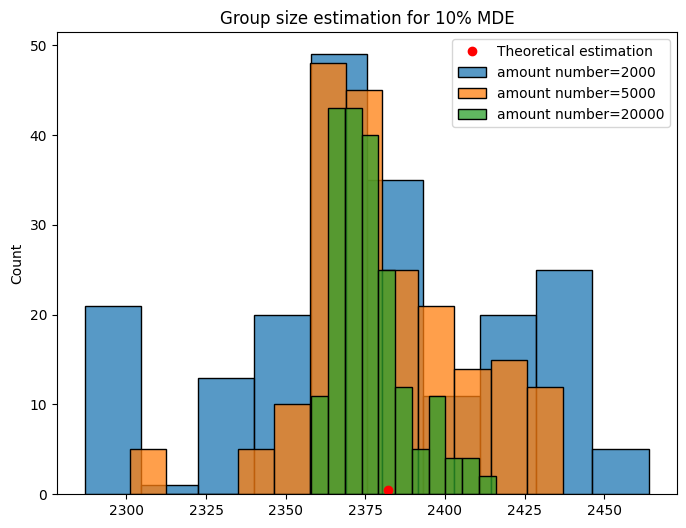
For small numbers of iterations interval parameter estimation is quite noisy, and one should be aware of it.
Experiment design based on a known retention rate value
And now we will calculate the experimental parameters using the known retantion rate value of 0.1.
[13]:
retention = 0.1
[14]:
# Create grid of MDEs and group sizes
# I and II type errros will have default values
effects = [1.01, 1.03, 1.05]
group_sizes = [20_000, 50_000, 100_000]
Design group sizes
[15]:
design_binary(to_design='size',
              prob_a=retention,
              method='theory',
              effects=effects)
[15]:
| Errors ($\alpha$, $\beta$) | (0.05; 0.2) |
|---|---|
| Effect | |
| 1.0% | 1419062 |
| 3.0% | 159059 |
| 5.0% | 57756 |
Design MDE values
[16]:
design_binary(to_design='effect',
              prob_a=retention,
              method='theory',
              sizes=group_sizes)
[16]:
| Errors ($\alpha$, $\beta$) | (0.05; 0.2) |
|---|---|
| Group sizes | |
| 20000 | 8.6% |
| 50000 | 5.4% |
| 100000 | 3.8% |
Design test power
[17]:
design_binary(to_design='power',
              prob_a=retention,
              method='theory',
              effects=effects,
              sizes=group_sizes)
[17]:
| Group sizes | 20000 | 50000 | 100000 | |
|---|---|---|---|---|
| $\alpha$ | Effect | |||
| 0.05 | 1.0% | 6.3% | 8.2% | 11.5% |
| 3.0% | 16.8% | 34.9% | 60.3% | |
| 5.0% | 37.8% | 74.1% | 95.8% |
Learn more
You can learn more information about how you can do A/B test design using Ambrosia
Check:
Binary design tools documentation
Main example of an experiment design using
Designerclass