Ambrosia data preprocessing tools overview¶

This example describes the data preprocessing methods which are implemented in the library. For the demonstration of these tools usage, synthetically generated one week data of daily content views by users is used.

Data processing tools are the number of classes that have the same access interface - they have set of implemented methods that are intuitive to the users:

fit - get the necessary for class parameters from the passed data
transform - make transformation of the passed data
fit_transform - combine the above two methods
get_params_dict - get a dict of fitted params
load_params_dict - set a dict of pre-fitted params
store_params - store fitted params to a file
load_params - load pre-fitted params from a file

Let’s take a look on some of preprocessing classes in the context of processing our user dataset.

[2]:

import numpy as np
import pandas as pd
import seaborn as sns

from ambrosia.preprocessing import (AggregatePreprocessor, RobustPreprocessor,
                                    IQRPreprocessor, LogTransformer,
                                    BoxCoxTransformer)

Load data

[3]:

data = pd.read_csv('../tests/test_data/week_metrics.csv')

[4]:

data.head()

[4]:

	id	gender	watched	sessions	day	platform
0	0	Male	28.440846	4	1	android
1	1	Female	1.825271	2	1	ios
2	2	Female	46.995606	0	1	web
3	3	Female	37.310264	1	1	ios
4	4	Female	147.513105	0	1	web

Data aggregation¶

In our task, we would like to first aggregate data by user in order, for example, to get a more reliable statistical picture of the views metric and get rid of intra-user the dependency.

For this we will use the AggregatePreprocessor class, which allows us to aggregate categorical and continuous variables in a convenient way.

The default aggregation behavior is set at instantiation time. However, when aggregating, we can always use the more detailed agg_params parameter, which sets own aggregation method for each metric.

[5]:

aggregator = AggregatePreprocessor(categorial_method='mode', real_method='sum')

Now fit aggregator and transform the data

[6]:

aggregator.fit_transform(dataframe=data,
                         groupby_columns='id',
                         real_cols=['watched', 'sessions'],
                         categorial_cols=['gender', 'platform'])

[6]:

	id	watched	sessions	gender	platform
0	0	772.597224	8	Male	ios
1	1	538.076739	15	Female	android
2	2	288.492353	20	Female	android
3	3	373.620408	9	Female	ios
4	4	630.238862	14	Female	ios
...	...	...	...	...	...
4995	4995	390.133588	14	Male	android
4996	4996	544.423724	25	Female	ios
4997	4997	204.713032	19	Male	android
4998	4998	1088.642872	25	Female	web
4999	4999	405.817078	11	Male	android

5000 rows × 5 columns

The instance is fitted now and we can see its parameters

[7]:

aggregator.get_params_dict()

[7]:

{'aggregation_params': {'watched': 'sum',
  'sessions': 'sum',
  'gender': 'mode',
  'platform': 'mode'},
 'groupby_columns': 'id'}

These parameters can be saved as a json file and loaded in the future for the same aggregation tasks. But first let’s refit the aggregator using detailed aggregation. You can use aliases for aggregation or pass pandas compatible methods.

[8]:

# Add extra column before
data['is_holiday'] = data['day'].apply(lambda x: 0 if x < 6 else 1)

[9]:

aggregator.fit_transform(
    data,
    groupby_columns=['id', 'is_holiday'],
    agg_params={
        'watched': 'sum',
        'sessions': 'max',
        'gender': 'simple',  # simple - choose the first possible value
        'platform': 'mode'
    })

[9]:

	id	is_holiday	watched	sessions	gender	platform
0	0	0	601.893096	4	Male	ios
1	0	1	170.704127	1	Male	android
2	1	0	327.533247	3	Female	web
3	1	1	210.543492	6	Female	ios
4	2	0	271.548875	7	Female	web
...	...	...	...	...	...	...
9995	4997	1	65.368574	2	Male	ios
9996	4998	0	1051.360035	4	Female	web
9997	4998	1	37.282837	10	Female	android
9998	4999	0	245.553217	6	Male	android
9999	4999	1	160.263861	2	Male	ios

10000 rows × 6 columns

Check and store instance parameters in a file

[10]:

aggregator.get_params_dict()

[10]:

{'aggregation_params': {'watched': 'sum',
  'sessions': 'max',
  'gender': 'simple',
  'platform': 'mode'},
 'groupby_columns': ['id', 'is_holiday']}

[11]:

aggregator.store_params('_examples_configs/aggregator.json')

Create new instance

[12]:

aggregator_loaded = AggregatePreprocessor()

Load parameters

[13]:

aggregator_loaded.load_params('_examples_configs/aggregator.json')

[14]:

aggregator_loaded.get_params_dict()

[14]:

{'aggregation_params': {'watched': 'sum',
  'sessions': 'max',
  'gender': 'simple',
  'platform': 'mode'},
 'groupby_columns': ['id', 'is_holiday']}

Aggregate data

[15]:

data_aggregated = aggregator_loaded.transform(data)

[16]:

data_aggregated.head()

[16]:

	id	is_holiday	watched	sessions	gender	platform
0	0	0	601.893096	4	Male	ios
1	0	1	170.704127	1	Male	android
2	1	0	327.533247	3	Female	web
3	1	1	210.543492	6	Female	ios
4	2	0	271.548875	7	Female	web

Cleaning the outliers¶

In many problems, we need to get rid of outliers in the data in order to make the results more reliable and applied statistical tests more sensitive.

For this purpose, the library contains 2 classes: RobustPreprocessor and IQRPreprocessor.

We will remove some rows from our aggregated data using these techniques.

`RobustPreprocessor`¶

The RobustPreprocessor removes objects that fall into the tails of the empirical distribution of the metrics that is estimaed form the passed data. The type of tail and its size for threshold calculation is specified by the user during fitting the data.

Let’s create an instance

[17]:

robust_transformer = RobustPreprocessor()

Fit transformer

[18]:

robust_transformer.fit(dataframe=data_aggregated,
                       column_names='watched',
                       alpha=0.01,
                       tail='right')

[18]:

<ambrosia.preprocessing.robust.RobustPreprocessor at 0x13ebc0c40>

Check fitted params

[19]:

robust_transformer.get_params_dict()

[19]:

{'tail': 'right',
 'column_names': ['watched'],
 'alpha': [0.01],
 'quantiles': [[1049.5734329308516]]}

Transform data (1% of rows will be removed, because this is the same dataframe)

[20]:

robust_transformer.transform(data_aggregated)

ambrosia LOGGER: Making right-tail robust transformation of columns ['watched']
                 with alphas = [0.01]
ambrosia LOGGER:

ambrosia LOGGER: Change Mean watched: 350.8333 ===> 342.2530
ambrosia LOGGER: Change Variance watched: 56929.6826 ===> 49971.0812
ambrosia LOGGER: Change IQR watched: 331.3509 ===> 325.2846
ambrosia LOGGER: Change Range watched: 1566.7685 ===> 1047.1196

[20]:

	id	is_holiday	watched	sessions	gender	platform
0	0	0	601.893096	4	Male	ios
1	0	1	170.704127	1	Male	android
2	1	0	327.533247	3	Female	web
3	1	1	210.543492	6	Female	ios
4	2	0	271.548875	7	Female	web
...	...	...	...	...	...	...
9994	4997	0	139.344458	6	Male	android
9995	4997	1	65.368574	2	Male	ios
9997	4998	1	37.282837	10	Female	android
9998	4999	0	245.553217	6	Male	android
9999	4999	1	160.263861	2	Male	ios

9900 rows × 6 columns

For all our preprocessing classes we have same methods for storing and loading parameters. This is useful to process the data in the future in the same way.

[21]:

robust_transformer.store_params('_examples_configs/robust.json')

Recreate instance

[22]:

del robust_transformer

robust_transformer = RobustPreprocessor()

Load params

[23]:

robust_transformer.load_params('_examples_configs/robust.json')

Transform data (we get the same transformation as before)

[24]:

robust_transformer.transform(data_aggregated)

ambrosia LOGGER: Making right-tail robust transformation of columns ['watched']
                 with alphas = [0.01]
ambrosia LOGGER:

ambrosia LOGGER: Change Mean watched: 350.8333 ===> 342.2530
ambrosia LOGGER: Change Variance watched: 56929.6826 ===> 49971.0812
ambrosia LOGGER: Change IQR watched: 331.3509 ===> 325.2846
ambrosia LOGGER: Change Range watched: 1566.7685 ===> 1047.1196

[24]:

	id	is_holiday	watched	sessions	gender	platform
0	0	0	601.893096	4	Male	ios
1	0	1	170.704127	1	Male	android
2	1	0	327.533247	3	Female	web
3	1	1	210.543492	6	Female	ios
4	2	0	271.548875	7	Female	web
...	...	...	...	...	...	...
9994	4997	0	139.344458	6	Male	android
9995	4997	1	65.368574	2	Male	ios
9997	4998	1	37.282837	10	Female	android
9998	4999	0	245.553217	6	Male	android
9999	4999	1	160.263861	2	Male	ios

9900 rows × 6 columns

The dispersion characteristics of the data have decreased.

`IQRPreprocessor`¶

The IQRPreprocessor class removes objects that go beyond the maximum and minimum values of the constructed boxplot based on the passed data with empirical distribution of the metrics.

Again create an instance

[25]:

iqr_transformer = IQRPreprocessor()

Fit (this time we will use two metrics)

[26]:

iqr_transformer.fit(dataframe=data_aggregated,
                    column_names=['watched', 'sessions'])

[26]:

<ambrosia.preprocessing.robust.IQRPreprocessor at 0x13ec32370>

Look at fitted params

[27]:

iqr_transformer.get_params_dict()

[27]:

{'column_names': ['watched', 'sessions'],
 'medians': [304.98240670946467, 4.0],
 'quartiles': [[161.81242236582537, 493.1633345302498], [2.0, 7.0]]}

Transform data

[28]:

data_aggregated = iqr_transformer.transform(data_aggregated)

ambrosia LOGGER: Making IQR transformation of columns ['watched', 'sessions']
ambrosia LOGGER:

ambrosia LOGGER: Change Mean watched: 350.8333 ===> 338.0876
ambrosia LOGGER: Change Variance watched: 56929.6826 ===> 47660.8027
ambrosia LOGGER: Change IQR watched: 331.3509 ===> 321.3204
ambrosia LOGGER: Change Range watched: 1566.7685 ===> 987.6670
ambrosia LOGGER:

ambrosia LOGGER: Change Mean sessions: 4.8478 ===> 4.5908
ambrosia LOGGER: Change Variance sessions: 12.5680 ===> 9.5394
ambrosia LOGGER: Change IQR sessions: 5.0000 ===> 4.0000
ambrosia LOGGER: Change Range sessions: 30.0000 ===> 14.0000

Check how many rows have been removed

[29]:

data_aggregated.shape

[29]:

(9662, 6)

Class instance parameters can be stored and loaded from a file as well as for other classes.

Metric tranformations¶

For some tasks, we may want to transform metrics, for example, to reduce the variance or make distribution shape more normal (however, be careful with this procedure, as you may lose the interpretability of the metrics).

For that purpose, we have implemented two common transformers: LogTransformer, BoxCoxTransformer.

We will demonstrate their work on our watched data.

`LogTransformer`¶

This transformer simply applied a logarithmic transformation to the metrics. Since it has the same interface as other classes, we still need to fit it to the data and it will fit only the names of the columns.

Create an instance

[30]:

log_transformer = LogTransformer()

Fit transformer

[31]:

log_transformer.fit(dataframe=data_aggregated, column_names=['watched'])

[31]:

<ambrosia.preprocessing.transformers.LogTransformer at 0x13ec3f580>

Transform data

[32]:

data_aggregated_logged = log_transformer.transform(data_aggregated)

Make sure that the variance of the metric has decreased after the transformation

[33]:

print('Original std:', data_aggregated.watched.std())
print('Log metric std:', data_aggregated_logged.watched.std())

Original std: 218.32484049843603
Log metric std: 0.827898247795576

Class instance parameters can be stored and loaded from a file.

`BoxCoxTransformer`¶

This class uses the Box-Cox transformation from the power transformation family and allows to make the data distribution more normal.

The lambda_ power parameter of the transformation is selected automatically during fitting.

Create an instance

[34]:

boxcox_transformer = BoxCoxTransformer()

Fit transformer

[35]:

boxcox_transformer.fit(dataframe=data_aggregated, column_names=['watched'])

[35]:

<ambrosia.preprocessing.transformers.BoxCoxTransformer at 0x13ec4a460>

Transform data

[36]:

boxcox_transformer.transform(data_aggregated)

[36]:

	id	is_holiday	watched	sessions	gender	platform
0	0	0	34.356077	4	Male	ios
1	0	1	18.974271	1	Male	android
2	1	0	25.887571	3	Female	web
3	1	1	20.991262	6	Female	ios
4	2	0	23.696137	7	Female	web
...	...	...	...	...	...	...
9994	4997	0	17.188778	6	Male	android
9995	4997	1	11.753853	2	Male	ios
9997	4998	1	8.726168	10	Female	android
9998	4999	0	22.590802	6	Male	android
9999	4999	1	18.402294	2	Male	ios

9662 rows × 6 columns

Check fitted parameters

[37]:

boxcox_transformer.get_params_dict()

[37]:

{'column_names': ['watched'], 'lambda_': [0.4314844480895849]}

Store them in a file

[38]:

boxcox_transformer.store_params('_examples_configs/boxcox_tranformer.json')

Create new instance

[39]:

boxcox_transformer_loaded = BoxCoxTransformer()

Load params

[40]:

boxcox_transformer_loaded.load_params(
    '_examples_configs/boxcox_tranformer.json')

Transform metric and compare distribution shape with the unchanged one

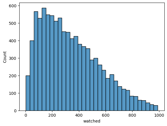
[41]:

sns.histplot(data_aggregated.watched)

[41]:

<AxesSubplot:xlabel='watched', ylabel='Count'>

../_images/pandas_examples_00_preprocessing_100_1.png

[42]:

sns.histplot(boxcox_transformer_loaded.transform(data_aggregated).watched)

[42]:

<AxesSubplot:xlabel='watched', ylabel='Count'>

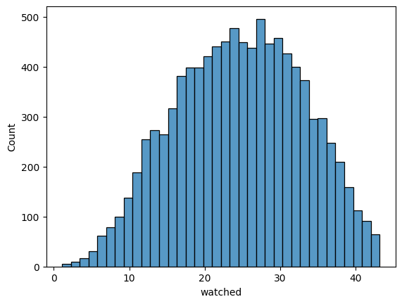
../_images/pandas_examples_00_preprocessing_101_1.png

Metric distribution becomes more normal

One note: for convenience, all transformers can apply their transformation directly to the passed dataframe, just set the inplace parameter to True in the corresponding transformation method.

Ambrosia preprocessing functionality is not limited to these classes

Check:

An overview of advanced metric transformation to learn about different methods for reducing variance
An overview of the Preprocessor class - a convenient chain pipeline transformer that combines almost all available preprocessing techniques in its methods
Ambrosia preprocessing modules documentation

Ambrosia data preprocessing tools overview¶

Data aggregation¶

Cleaning the outliers¶

RobustPreprocessor¶

IQRPreprocessor¶

Metric tranformations¶

LogTransformer¶

BoxCoxTransformer¶

`RobustPreprocessor`¶

`IQRPreprocessor`¶

`LogTransformer`¶

`BoxCoxTransformer`¶